Signals & Systems Cheatsheet – Transform Formulas & Graphs

Introduction

Signals & Systems is one of the most important subjects in Electronics & Communication Engineering (ECE), forming the foundation for advanced courses like DSP, Communication Systems, and Control Engineering.

However, students often struggle during exams because the subject involves a wide variety of formulas, properties, and transform equations. To make things easier, we’ve created this Signals & Systems Cheatsheet — a quick revision guide with transform formulas, graphical representations, and key properties.

This article is designed for BTech students, competitive exam aspirants (GATE, ESE), and anyone preparing for quick revisions. Bookmark this page and use it as your last-minute exam resource.

Basics of Signals & Systems

Before diving into formulas, let’s quickly revise the basics.

Types of Signals

• Continuous-Time Signal (CTS) — Defined at every instant of time.
• Discrete-Time Signal (DTS) — Defined only at discrete time intervals.
• Periodic Signal — Repeats after a fixed time period.
• Aperiodic Signal — Does not repeat.
• Deterministic Signal — Can be described by a mathematical expression.
• Random Signal — Cannot be precisely predicted.

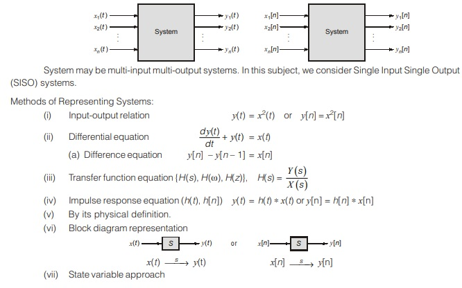
Types of Systems

• Linear vs Non-Linear
• Time-Invariant vs Time-Variant
• Causal vs Non-Causal
• Stable vs Unstable

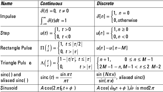
Commonly Used Signals and Their Graphs

Unit Impulse Signal (δ(t))

• Defined as:
  • δ(t) = 1 when t = 0
  • δ(t) = 0 when t ≠ 0

Unit Step Signal (u(t))

• u(t) = 1 for t ≥ 0, and 0 for t < 0

Ramp Signal (r(t))

• r(t) = t for t ≥ 0, else 0

Exponential Signal

• x(t) = e^(at), continuous exponential function

Sinusoidal Signal

• x(t) = A sin(ωt + θ)

Transform Formulas Cheatsheet

One of the most crucial parts of Signals & Systems is mastering the transform techniques. Below are the key transforms:

Fourier Transform (FT)

Definition:

X(ω) = ∫ x(t) e^(-jωt) dt

Common Fourier Transform Pairs:

• δ(t) ⇔ 1
• u(t) ⇔ 1/(jω) + πδ(ω)
• e^(-at)u(t) ⇔ 1/(a + jω), Re(a) > 0
• cos(ω₀t) ⇔ π[δ(ω – ω₀) + δ(ω + ω₀)]
• sin(ω₀t) ⇔ jπ[δ(ω + ω₀) – δ(ω – ω₀)]

Properties:

• Linearity
• Time Shifting
• Frequency Shifting
• Time Scaling
• Convolution in Time ⇔ Multiplication in Frequency

Laplace Transform (LT)

Definition:

X(s) = ∫ x(t) e^(-st) dt

Common Laplace Transform Pairs:

• δ(t) ⇔ 1
• u(t) ⇔ 1/s
• e^(-at)u(t) ⇔ 1/(s + a)
• sin(ωt)u(t) ⇔ ω/(s² + ω²)
• cos(ωt)u(t) ⇔ s/(s² + ω²)

Properties:

• Linearity
• Time Shifting
• Differentiation in Time ⇔ Multiplication by s
• Convolution ⇔ Multiplication
• Initial Value Theorem: x(0⁺) = lim(s→∞) sX(s)
• Final Value Theorem: x(∞) = lim(s→0) sX(s)

Z-Transform (ZT)

Definition:

X(z) = Σ [x(n) z^(-n)], n = -∞ to ∞

Common Z-Transform Pairs:

• δ[n] ⇔ 1
• u[n] ⇔ 1/(1 – z^(-1)), |z| > 1
• a^n u[n] ⇔ 1/(1 – az^(-1)), |z| > |a|
• sin(ω₀n)u[n] ⇔ (z sin ω₀)/(z² – 2z cos ω₀ + 1)
• cos(ω₀n)u[n] ⇔ (z² – z cos ω₀)/(z² – 2z cos ω₀ + 1)

Properties:

• Linearity
• Time Shifting
• Scaling in z-Domain
• Differentiation Property

Comparison Between Transforms

Feature	Fourier Transform	Laplace Transform	Z Transform
Domain	Frequency (ω)	Complex (s)	Complex (z)
Used For	Frequency Analysis	Continuous-time Systems	Discrete-time Systems
ROC Importance	No	Yes	Yes
Application	Signal Spectrum	System Stability	Digital Filters

Key Graphs for Signals & Systems

Students are often asked to draw graphs of signals and transforms in exams. Below are the must-know ones:

• Unit step, ramp, impulse graphs
• Sinusoidal signal spectrum
• Exponential signal decay/growth
• Fourier Transform magnitude & phase spectrum examples
• Pole-zero plots in Laplace and Z-domain

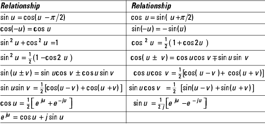
Tips for Remembering Transform Formulas

• Always group transforms under Impulse, Step, Exponential, Sinusoidal.
• Revise properties more than formulas (most exam questions are property-based).
• Use symmetry properties of Fourier to save time.
• Practice pole-zero plots for Laplace & Z-Transform.

Quick Revision Formula Sheet (Summary)

• Fourier: δ(t) ⇔ 1, u(t) ⇔ 1/(jω) + πδ(ω)
• Laplace: u(t) ⇔ 1/s, e^(-at) ⇔ 1/(s+a)
• Z-Transform: u[n] ⇔ 1/(1 – z⁻¹), a^n u[n] ⇔ 1/(1 – az⁻¹)

FAQs on Signals & Systems Cheatsheet

1. Why are transforms important in Signals & Systems?

Transforms like Fourier, Laplace, and Z are essential because they convert complex time-domain signals into simpler frequency or complex-domain representations, making analysis easier.

2. Which transform should I use for discrete signals?

For discrete-time signals, Z-Transform is preferred as it simplifies digital system analysis.

3. Is Fourier Transform used in real-life applications?

Yes. It is widely used in communication systems, image processing, audio signal analysis, and filtering.

4. How to quickly revise Signals & Systems before exams?

Use a cheatsheet with formulas and graphs (like this one), focus on properties, and practice previous year question papers.

5. What is the difference between Laplace and Fourier Transform?

Fourier deals mainly with frequency-domain representation, while Laplace is more general, handling both growth and decay behaviors with its Region of Convergence (ROC).

Conclusion

Signals & Systems may look intimidating, but once you break it into basic signals, transforms, and properties, it becomes very manageable. This cheatsheet with formulas, graphs, and properties is perfect for last-minute revision before exams.

Keep revising the transforms daily, and use this page as your quick-access formula sheet whenever you need.

[CTA BUTTON: Download Full PDF Cheatsheet — Link: https://btechcheatsheets.com/download-signals-systems-cheatsheet]